Siamese Network on MNIST Dataset

Introduction

Siamese Network is a semi-supervised learning network which produces the embedding feature representation for the input. By introducing multiple input channels in the network and appropriate loss functions, the Siamese Network is able to learn to represent similar inputs with similar embedding features and represent different inputs with different embedding features.

Usually, the embedding feature is a high dimensional vector. The similarity of the embedding features is usually represented by the Euclidean distance in the high dimensional space.

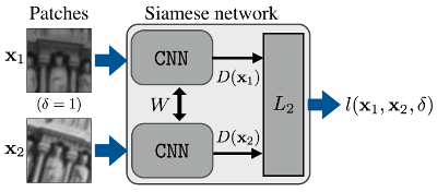
Here is a typical Siamese Network with two input channels (Deep Convolutional Feature Point Descriptors). The two identical sister networks, which are Convolutional Neural Networks (CNN) in this case, share the same weights. In addition to CNN, the architecture generally could be any neural networks. It should be noted that the two sister networks could be of the same or different architecture. Even if the two sister networks are of the same architecture, they do not have to share weights but use distinct weights. Usually, if the inputs are of different “type”, the sister networks usually use different architectures or use distinct weights for the same architecture.

The two statue images were input into the two channels of the Siamese Network. Because the two inputs are the same kind of inputs (image of objects), the two sister CNNs shares weights between each other. The L2 distance (Euclidean distance) of the outputs of the two channels were calculated and subjected to the loss function $$l(x_1, x_2, \delta)$$ minimization. Here, the loss function is a function called contrastive loss function first proposed by Yann LeCunn (Dimensionality Reduction by Learning an Invariant Mapping), which I will elaborate in the following sections. If the two images are representing the same object, the two outputs should be very close in the higher dimensional space, i.e., small L2 distance. Otherwise, the two outputs should be very far away from each other in the higher dimensional space, i.e., large L2 distance.

I will first give an example of my implementation of the Siamese Network using identical architectures with shared weights on MNIST dataset. Followed by a more complex example using different architectures or different weights with the same architecture.

Siamese Network on MNIST Dataset

The whole Siamese Network implementation was wrapped as Python object. One can easily modify the counterparts in the object to achieve more advanced goals, such as replacing FNN to more advanced neural networks, changing loss functions, etc. See the Siamese Network on MNIST in my GitHub repository.

The sister networks I used for the MNIST dataset are three layers of FNN. All the implementations of the network are nothing special compared to the implementations of other networks in TensorFlow, except for three caveats.

Share Weights Between Networks

Use scope.reuse_variables() to tell TensorFlow the variables used in the scope for output_1 needs to be reused for output_2. Although I have not tested, the variables in the scope could be reused as many times as possible as long as scope.reuse_variables() is stated after the usage of the variables.

def network_initializer(self):
    # Initialze neural network
    with tf.variable_scope("siamese") as scope:
        output_1 = self.network(self.tf_input_1)
        # Share weights
        scope.reuse_variables()
        output_2 = self.network(self.tf_input_2)
    return output_1, output_2

Implementation of the Contrastive Loss

We typically use Contrastive Loss function $L(I_1, I_2, l)$ in Siamese Network with two input channels.

$$
L(I_1, I_2, l) = ld(I_1, I_2)^2 + (1-l)\max(m - d(I_1, I_2), 0)^2
$$

$I_1$ is the high-dimensional feature vector for input 1, and $I_2$ is the high-dimensional feature vector for input 2. $l$ is a binary-valued correspondence variable that indicates whether the two feature vector pair match ($l = 1$) or not ($l = 0$). $d(I_1, I_2)$ is the Euclidean distance of $I_1$ and $I_2$. $m$ ($m > 0$) is the margin for non-matched feature vector pair. To understand the margin $m$, when the two feature vector do not pair, $l = 0$, $L(I_1, I_2, l = 0) = \max(m - d(I_1, I_2), 0)^2$. To minimize the loss, $d(I_1, I_2)$ could neither be too large nor too small, but close to the margin $m$. If the dimension of feature vector is fixed, increasing the value of margin $m$ may allow better separation of data clusters, but the training time may also increase given other parameters are fixed.

However, in the implementation, using this exact Contrastive Loss function will cause some problems. For example, the loss will keep decreasing during training, but suddenly became NaN which does not make sense at first glance. This is because the gradient property for this Contrastive Loss function is not very good.

Let’s see an example.

Suppose $I_1 = (a_1, a_2)$, $I_2 = (b_1, b_2)$, then $d(I_1, I_2) = \sqrt{(a_1-b_1)^2 + (a_2-b_2)^2}$. We then calculate its partial derivative to $a_1$.

$$\frac{\partial d(I_1, I_2)}{\partial a_1} = \frac{a_1 - b_1}{\sqrt{(a_1-b_1)^2 + (a_2-b_2)^2}}$$

When $a_1 = b_1$ and $a_2 = b_2$, or $I_1$ and $I_2$ are extremely close to each other, this derivative is likely to be NaN. This derivative is absolutely required for the training cases whose $l = 0$.

Although the chance of happening during training might be low since the label $l$ suggesting that $I_1$ and $I_2$ should be divergent, there is still a chance that $I_1$ and $I_2$ are extremely close while $l = 0$. Once this happens once, the loss function should always give NaN for the loss and derivatives.

To overcome this bad property, I added a small number to the Euclidean distance when $l = 0$, making the Euclidean distance never be zero. Formally, the Contrastive Loss function becomes

$$
L(I_1, I_2, l) = ld(I_1, I_2)^2 + (1-l)\max(m - d’(I_1, I_2), 0)^2
$$

Where $d(I_1, I_2)$ is the Euclidean distance of $I_1$ and $I_2$, $d’(I_1, I_2) = \sqrt{d(I_1, I_2)^2 + \lambda}$. Here I used $\lambda = 10^{-6}$ in this case.

def loss_contrastive(self, margin = 5.0):
    # Define loss function
    with tf.variable_scope("loss_function") as scope:
        labels = self.tf_label
        # Euclidean distance squared
        eucd2 = tf.pow(tf.subtract(self.output_1, self.output_2), 2, name = 'eucd2')
        eucd2 = tf.reduce_sum(eucd2, 1)
        # Euclidean distance
        # We add a small value 1e-6 to increase the stability of calculating the gradients for sqrt
        # See https://github.com/tensorflow/tensorflow/issues/4914
        eucd = tf.sqrt(eucd2 + 1e-6, name = 'eucd')
        # Loss function
        loss_pos = tf.multiply(labels, eucd2, name = 'constrastive_loss_1')
        loss_neg = tf.multiply(tf.subtract(1.0, labels), tf.pow(tf.maximum(tf.subtract(margin, eucd), 0), 2), name = 'constrastive_loss_2')
        loss = tf.reduce_mean(tf.add(loss_neg, loss_pos), name = 'constrastive_loss')
    return loss

Choice of the Optimizers

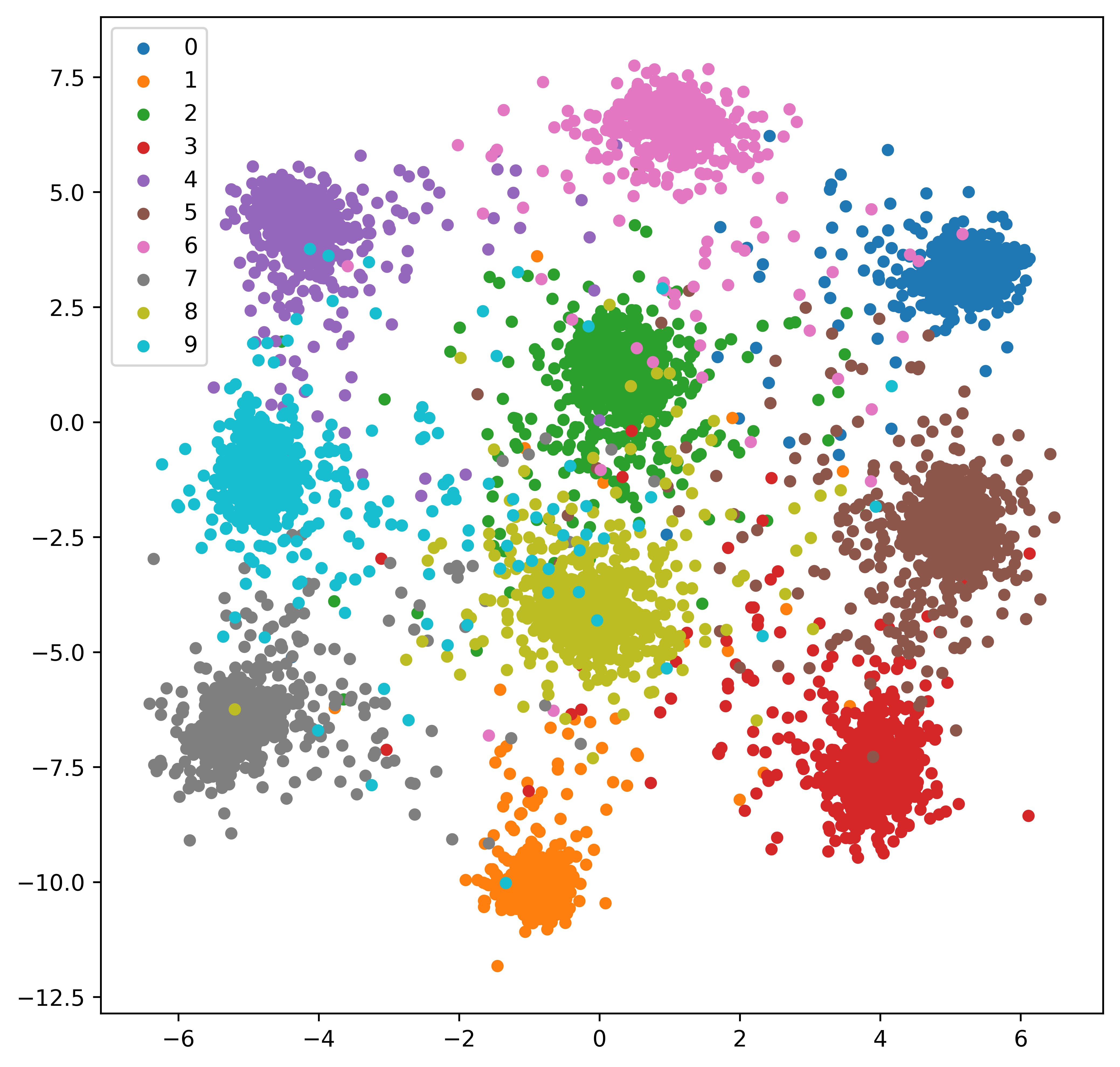
Different optimizers tend to have different training effects. I tried AdamOptimizer, and I found although the feature vectors got separated, the cluster shape was spindly. I later used GradientDescentOptimizer, the cluster shape became circle instead.

def optimizer_initializer(self):
    # Initialize optimizer
    # AdamOptimizer and GradientDescentOptimizer has different effect on the final results
    # GradientDescentOptimizer is probably better than AdamOptimizer in Siamese Network
    #optimizer = tf.train.AdamOptimizer(LEARNING_RATE).minimize(self.loss)
    optimizer = tf.train.GradientDescentOptimizer(LEARNING_RATE).minimize(self.loss)
    return optimizer

Test Result

Siamese Network with Two Data Sources

As I mentioned above, Siamese Network could also be used to train data inputs of different “types”. One such example is described in the paper “Satellite image-based localization via learned embeddings”. The authors of the paper used VGG16 network for both Siamese channels, but unlike the MNIST example, the weights of VGG16 network is not shared because one input image is camera photo and the other input image is a satellite map image.