Simple Illustration of Programmable Backpropagation

Backpropagation Derivation

Backpropagation is always one of my knowledge weaknesses in machine learning. I have understood it many times. However, I always forgot how it really works but simply remember it is basically about the multivariable chain rules. I clearly remember that Andrew Ng once joked he sometimes cannot remember how backpropagation works so he often had to understand backpropagation again before he gave lectures in machine learning courses. Even if I refresh my mind by reading some related materials, I never understood why such tedious and complicated calculus could be programmable in our machine learning tools when we are working on neural networks.

If you know how to calculate \(\frac{\partial{e}}{\partial{b}}\) in the following figure, you basically know how to do backpropagation.
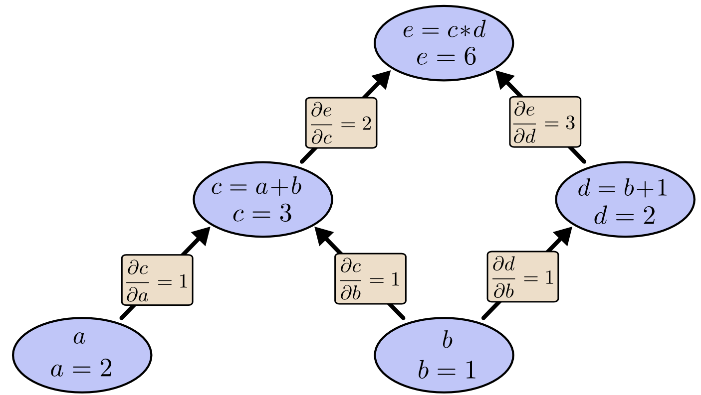
Backpropagation

Here is a very simple and good illustration of the backpropagation. However, these materials are often over-simplified. The network they provided is not even the ordinary neural network we are using nowadays. Not even mention including the activation functions.

Here, I neatly presented the workflow of backpropagation so that people could easily figure out the programmable logic inside the derivations. It is extremely tedious to type equations in MathJax. So I finally chose to use Word and transformed the file to pdf for you guys to download.

You can download my simple illustration of programmable backpropagation here.

Backpropagation was always like a black box when I was working on machine learning tasks. I hope these materials could always remind me the mechanism of backpropagation and the importance of mathematics in computer science.

Backpropagation Implementation

Here is a code example of the neural network backpropagation. In case the author makes changes or removes the contents, you may also download it from my site. The author also wrote blogs (page 1, page 2) on the implementation of this backpropagation to solve classification problems.

Although it might twist your brain, the author’s implementation has exactly the same logic to mine (He specifically used sigmoid function as activation function and least sum-of-squares function as loss function). The implementation was very neat, which only used Numpy. I think it would take me a very long time if I am going to write it myself.

The key codes of backpropagation are as follows:

1
2
3
4
5
6
7
8
9
10
11
12
13
14
15
16
17
18
19
20
21
22
23
24
25
26
27
28
29
30
31
32
33
34
35
36
37
38
39
40
41
42
43
44
45
46
47
48
49
50
51
52
53
54
55
56
57
58
59
60
    def update_mini_batch(self, mini_batch, eta):
"""Update the network's weights and biases by applying
gradient descent using backpropagation to a single mini batch.
The ``mini_batch`` is a list of tuples ``(x, y)``, and ``eta``
is the learning rate."""
nabla_b = [np.zeros(b.shape) for b in self.biases]
nabla_w = [np.zeros(w.shape) for w in self.weights]
for x, y in mini_batch:
delta_nabla_b, delta_nabla_w = self.backprop(x, y)
nabla_b = [nb+dnb for nb, dnb in zip(nabla_b, delta_nabla_b)]
nabla_w = [nw+dnw for nw, dnw in zip(nabla_w, delta_nabla_w)]
self.weights = [w-(eta/len(mini_batch))*nw
for w, nw in zip(self.weights, nabla_w)]
self.biases = [b-(eta/len(mini_batch))*nb
for b, nb in zip(self.biases, nabla_b)]

def backprop(self, x, y):
"""Return a tuple ``(nabla_b, nabla_w)`` representing the
gradient for the cost function C_x. ``nabla_b`` and
``nabla_w`` are layer-by-layer lists of numpy arrays, similar
to ``self.biases`` and ``self.weights``."""
nabla_b = [np.zeros(b.shape) for b in self.biases]
nabla_w = [np.zeros(w.shape) for w in self.weights]
# feedforward
activation = x
activations = [x] # list to store all the activations, layer by layer
zs = [] # list to store all the z vectors, layer by layer
for b, w in zip(self.biases, self.weights):
z = np.dot(w, activation)+b
zs.append(z)
activation = sigmoid(z)
activations.append(activation)
# backward pass
delta = self.cost_derivative(activations[-1], y) * \
sigmoid_prime(zs[-1])
nabla_b[-1] = delta
nabla_w[-1] = np.dot(delta, activations[-2].transpose())
# Note that the variable l in the loop below is used a little
# differently to the notation in Chapter 2 of the book. Here,
# l = 1 means the last layer of neurons, l = 2 is the
# second-last layer, and so on. It's a renumbering of the
# scheme in the book, used here to take advantage of the fact
# that Python can use negative indices in lists.
for l in xrange(2, self.num_layers):
z = zs[-l]
sp = sigmoid_prime(z)
delta = np.dot(self.weights[-l+1].transpose(), delta) * sp
nabla_b[-l] = delta
nabla_w[-l] = np.dot(delta, activations[-l-1].transpose())
return (nabla_b, nabla_w)

#### Miscellaneous functions
def sigmoid(z):
"""The sigmoid function."""
return 1.0/(1.0+np.exp(-z))

def sigmoid_prime(z):
"""Derivative of the sigmoid function."""
return sigmoid(z)*(1-sigmoid(z))

His weights and biases matrices were organized in this way by the way.

1
2
3
4
5
6
7
8
9
10
11
12
13
14
15
16
17
18
class Network(object):

def __init__(self, sizes):
"""The list ``sizes`` contains the number of neurons in the
respective layers of the network. For example, if the list
was [2, 3, 1] then it would be a three-layer network, with the
first layer containing 2 neurons, the second layer 3 neurons,
and the third layer 1 neuron. The biases and weights for the
network are initialized randomly, using a Gaussian
distribution with mean 0, and variance 1. Note that the first
layer is assumed to be an input layer, and by convention we
won't set any biases for those neurons, since biases are only
ever used in computing the outputs from later layers."""
self.num_layers = len(sizes)
self.sizes = sizes
self.biases = [np.random.randn(y, 1) for y in sizes[1:]]
self.weights = [np.random.randn(y, x)
for x, y in zip(sizes[:-1], sizes[1:])]

I remember that when I was taking GRE test years ago, there is a topic of “human beings become stupid as the technology develops”. I might agree with it to some extent, because using too many tools when we are coding or doing numerical analysis makes us stupid.

I have seen many deep learning codes which only use Numpy, and I really admire them very much. We are actually over-using the autograds functions in modern tools, such as Tensorflow. Finally, the learning algorithm we developed becomes a black box, which is pretty bad. There are other reasons, in addition to autograds, why we are using such modern tools.

We have to keep in mind that mathematics always comes first even if we are computer scientists.

Simple Illustration of Programmable Backpropagation

https://leimao.github.io/blog/Programmable-Backpropagation/

Author

Lei Mao

Posted on

05-17-2017

Updated on

05-17-2017

Licensed under


Comments